Homework-8
Juliana Dau
2025-03-19
1. Using sample Code
library(ggplot2)
library(MASS)
z <- rnorm(n=3000,mean=0.2)
z <- data.frame(1:3000,z)
names(z) <- list("ID","myVar")
z <- z[z$myVar>0,]
str(z)## 'data.frame': 1682 obs. of 2 variables:
## $ ID : int 1 3 6 7 8 10 12 13 14 15 ...
## $ myVar: num 0.9892 0.7955 2.3365 0.0612 1.4703 ...summary(z$myVar)## Min. 1st Qu. Median Mean 3rd Qu. Max.
## 0.00401 0.36955 0.75814 0.88224 1.26338 3.71709#Histogram. #Observation: R studio indicated that some were deprecated and sugested to change size to linewith so I did it.
p1 <- ggplot(data=z, aes(x=myVar, y=..density..)) +
  geom_histogram(color="grey60",fill="cornsilk",linewidth=0.2)
print(p1)
## Warning: The dot-dot notation (`..density..`) was deprecated in ggplot2 3.4.0.
## ℹ Please use `after_stat(density)` instead.
## This warning is displayed once every 8 hours.
## Call `lifecycle::last_lifecycle_warnings()` to see where this warning was
## generated.## `stat_bin()` using `bins = 30`. Pick better value with `binwidth`.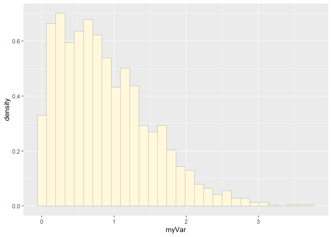
#Empirical density curve
p1 <-  p1 +  geom_density(linetype="dotted",linewidth=0.75)
print(p1)
## `stat_bin()` using `bins = 30`. Pick better value with `binwidth`.
#Maximum likelihood parameters for normal
normPars <- fitdistr(z$myVar,"normal")
print(normPars)
## mean sd
## 0.88223649 0.63442715
## (0.01546923) (0.01093840)str(normPars)## List of 5
## $ estimate: Named num [1:2] 0.882 0.634
## ..- attr(*, "names")= chr [1:2] "mean" "sd"
## $ sd : Named num [1:2] 0.0155 0.0109
## ..- attr(*, "names")= chr [1:2] "mean" "sd"
## $ vcov : num [1:2, 1:2] 0.000239 0 0 0.00012
## ..- attr(*, "dimnames")=List of 2
## .. ..$ : chr [1:2] "mean" "sd"
## .. ..$ : chr [1:2] "mean" "sd"
## $ n : int 1682
## $ loglik : num -1621
## - attr(*, "class")= chr "fitdistr"normPars$estimate["mean"]## mean
## 0.8822365#Plot normal probability density
meanML <- normPars$estimate["mean"]
sdML <- normPars$estimate["sd"]

xval <- seq(0,max(z$myVar),len=length(z$myVar))

 stat <- stat_function(aes(x = xval, y = ..y..), fun = dnorm, colour="red", n = length(z$myVar), args = list(mean = meanML, sd = sdML))
 p1 + stat
## `stat_bin()` using `bins = 30`. Pick better value with `binwidth`.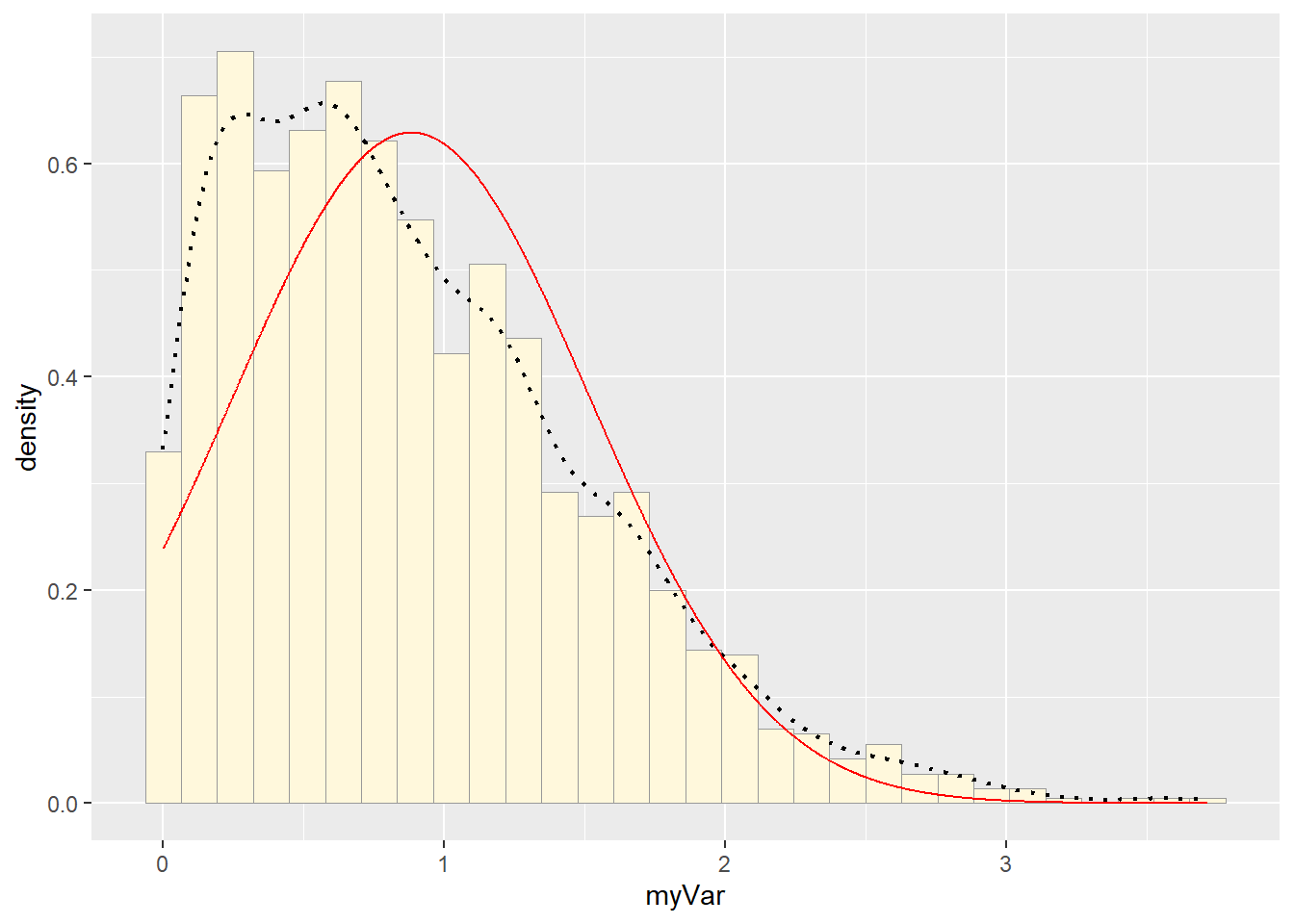
#Plot exponential probability density
expoPars <- fitdistr(z$myVar,"exponential")
rateML <- expoPars$estimate["rate"]

stat2 <- stat_function(aes(x = xval, y = ..y..), fun = dexp, colour="blue", n = length(z$myVar), args = list(rate=rateML))
 p1 + stat + stat2
## `stat_bin()` using `bins = 30`. Pick better value with `binwidth`.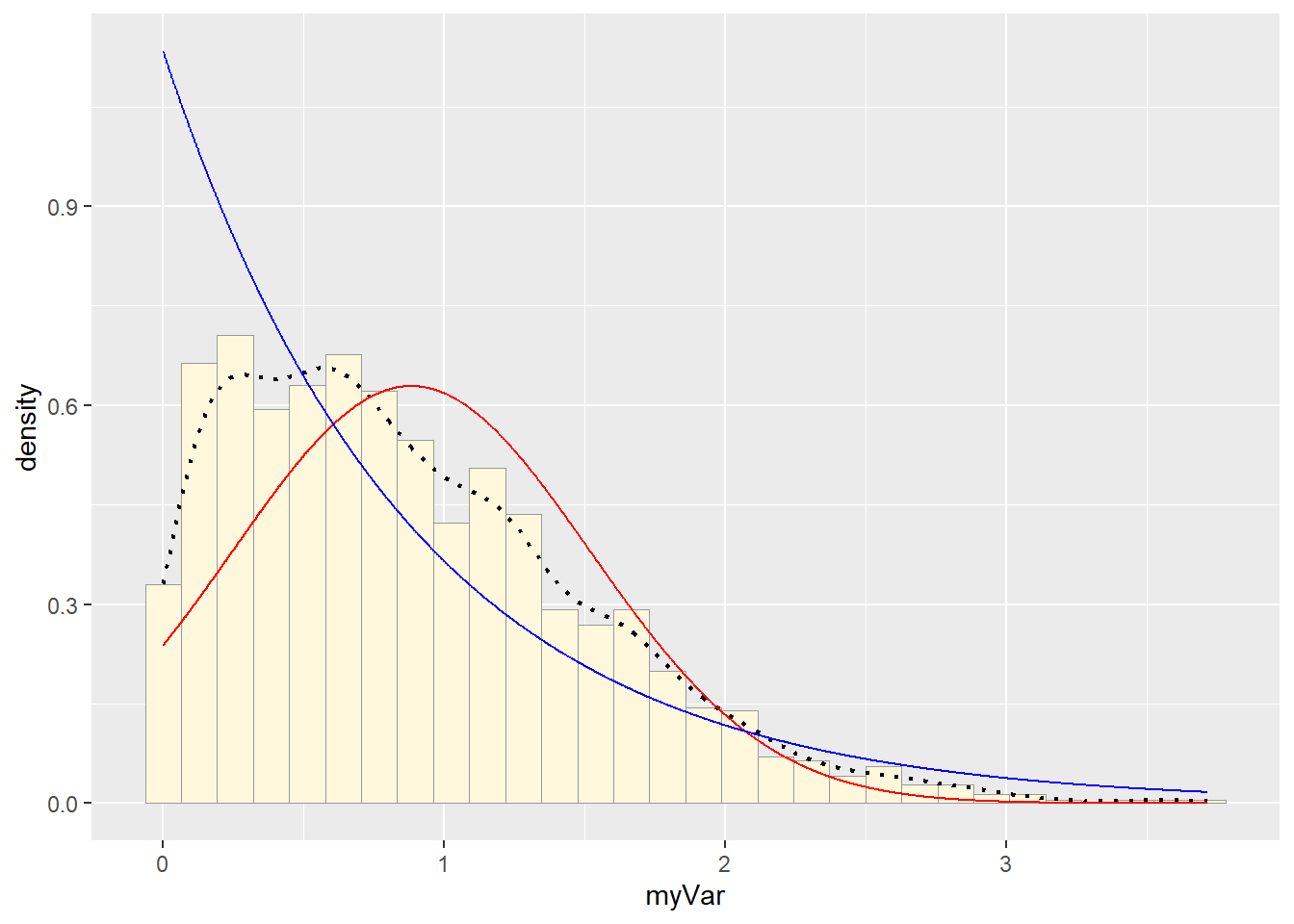 #Plot uniform probability density
stat3 <- stat_function(aes(x = xval, y = ..y..), fun = dunif, colour="darkgreen", n = length(z$myVar), args = list(min=min(z$myVar), max=max(z$myVar)))
 p1 + stat + stat2 + stat3
## `stat_bin()` using `bins = 30`. Pick better value with `binwidth`.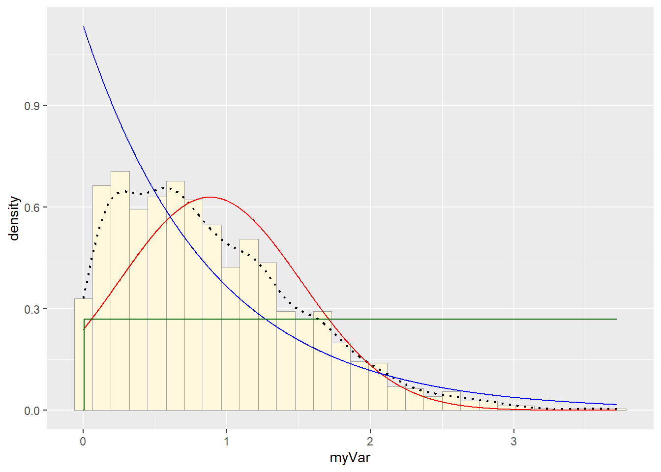 #Plot gamma probability density
gammaPars <- fitdistr(z$myVar,"gamma")## Warning in densfun(x, parm[1], parm[2], ...): NaNs produzidos
## Warning in densfun(x, parm[1], parm[2], ...): NaNs produzidos
## Warning in densfun(x, parm[1], parm[2], ...): NaNs produzidos
## Warning in densfun(x, parm[1], parm[2], ...): NaNs produzidos
## Warning in densfun(x, parm[1], parm[2], ...): NaNs produzidos
## Warning in densfun(x, parm[1], parm[2], ...): NaNs produzidos
## Warning in densfun(x, parm[1], parm[2], ...): NaNs produzidosshapeML <- gammaPars$estimate["shape"]
rateML <- gammaPars$estimate["rate"]
stat4 <- stat_function(aes(x = xval, y = ..y..), fun = dgamma, colour="brown", n = length(z$myVar), args = list(shape=shapeML, rate=rateML))
p1 + stat + stat2 + stat3 + stat4## `stat_bin()` using `bins = 30`. Pick better value with `binwidth`. #Plot beta probability density
pSpecial <- ggplot(data=z, aes(x=myVar/(max(myVar + 0.1)), y=..density..)) +
  geom_histogram(color="grey60",fill="cornsilk",size=0.2) +
  xlim(c(0,1)) +
  geom_density(size=0.75,linetype="dotted")
## Warning: Using `size` aesthetic for lines was deprecated in ggplot2 3.4.0.
## ℹ Please use `linewidth` instead.
## This warning is displayed once every 8 hours.
## Call `lifecycle::last_lifecycle_warnings()` to see where this warning was
## generated.betaPars <- fitdistr(x=z$myVar/max(z$myVar + 0.1),start=list(shape1=1,shape2=2),"beta")## Warning in densfun(x, parm[1], parm[2], ...): NaNs produzidos## Warning in densfun(x, parm[1], parm[2], ...): NaNs produzidos
## Warning in densfun(x, parm[1], parm[2], ...): NaNs produzidos
## Warning in densfun(x, parm[1], parm[2], ...): NaNs produzidosshape1ML <- betaPars$estimate["shape1"]
shape2ML <- betaPars$estimate["shape2"]
statSpecial <- stat_function(aes(x = xval, y = ..y..), fun = dbeta, colour="orchid", n = length(z$myVar), args = list(shape1=shape1ML,shape2=shape2ML))
pSpecial + statSpecial## `stat_bin()` using `bins = 30`. Pick better value with `binwidth`.## Warning: Removed 2 rows containing missing values or values outside the scale range
## (`geom_bar()`).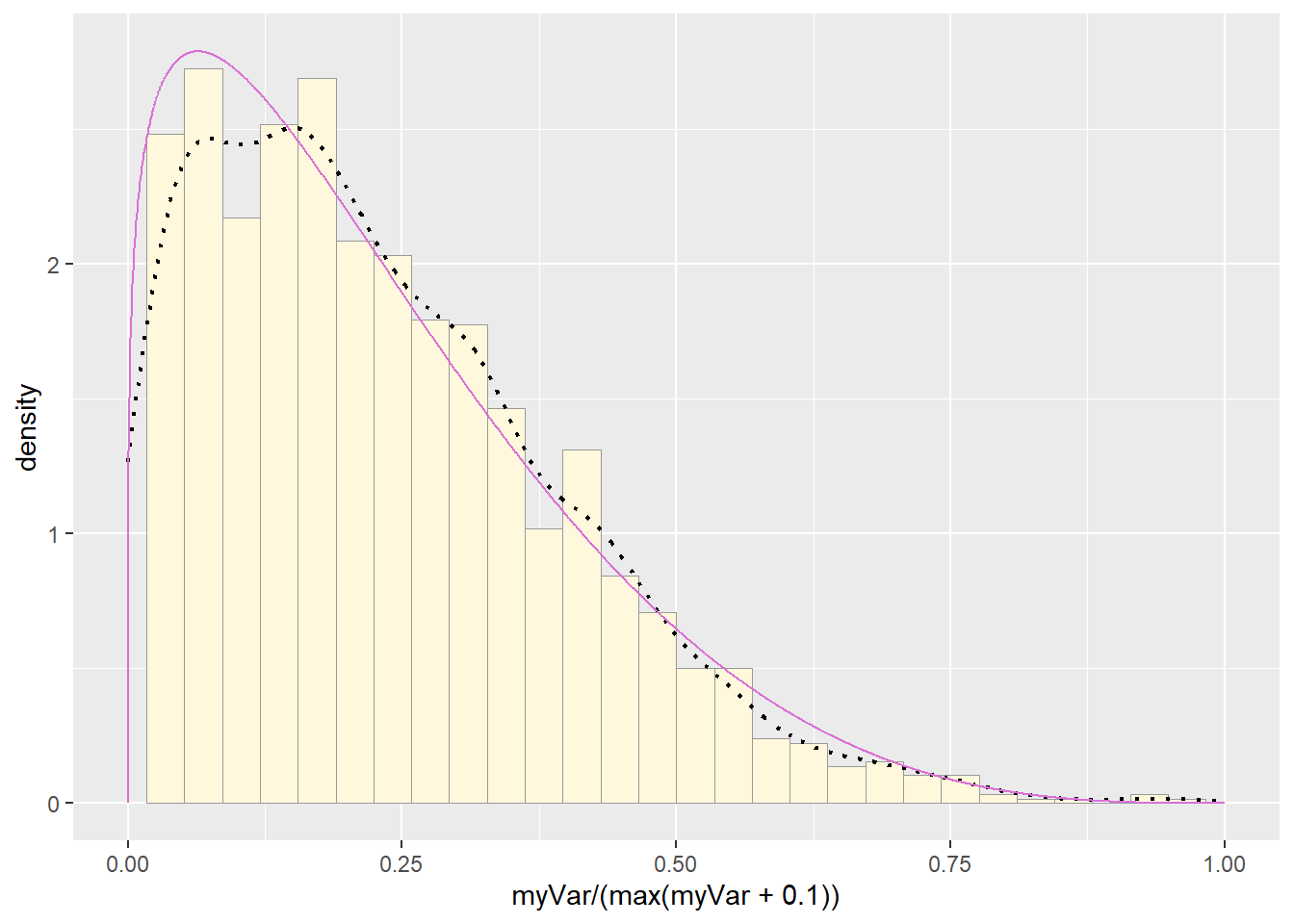
Visually gamma or beta probability density seemed to be the better fit.
2. Using Own data/External data
#Similar to Homework 6 used the quantification of surfactant protein C (SPC) found in the bronchoalveolar lavage fluid across 16 animals.
Z <- read.table("SPC.quantification.homework8.csv",header=TRUE,sep=",")
str(Z)## 'data.frame': 16 obs. of 1 variable:
## $ SPC: int 23001 19049 7023 12627 20170 13906 16829 29307 22435 30349 ...summary(Z)## SPC
## Min. : 7023
## 1st Qu.:16650
## Median :22013
## Mean :24188
## 3rd Qu.:31703
## Max. :42109#Histogram.
p2 <- ggplot(data=Z, aes(x=SPC, y=..density..)) +
geom_histogram(color="grey60",fill="cornsilk",linewidth=0.2)
print(p2)## `stat_bin()` using `bins = 30`. Pick better value with `binwidth`.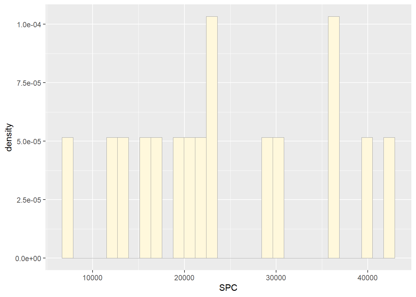
#Empirical density curve
p2 <- p2 + geom_density(linetype="dotted",size=0.75)
print(p2)## `stat_bin()` using `bins = 30`. Pick better value with `binwidth`.
#Maximum likelihood parameters for normal
normPars2 <- fitdistr(Z$SPC,"normal")
print(normPars2)## mean sd
## 24188.375 10104.202
## ( 2526.051) ( 1786.188)str(normPars2)## List of 5
## $ estimate: Named num [1:2] 24188 10104
## ..- attr(*, "names")= chr [1:2] "mean" "sd"
## $ sd : Named num [1:2] 2526 1786
## ..- attr(*, "names")= chr [1:2] "mean" "sd"
## $ vcov : num [1:2, 1:2] 6380932 0 0 3190466
## ..- attr(*, "dimnames")=List of 2
## .. ..$ : chr [1:2] "mean" "sd"
## .. ..$ : chr [1:2] "mean" "sd"
## $ n : int 16
## $ loglik : num -170
## - attr(*, "class")= chr "fitdistr"normPars2$estimate["mean"] ## mean
## 24188.38#Plot normal probability density
meanML <- normPars2$estimate["mean"]
sdML <- normPars2$estimate["sd"]
xval <- seq(0,max(Z$SPC),len=length(Z$SPC))
stat <- stat_function(aes(x = xval, y = ..y..), fun = dnorm, colour="red", n = length(Z$SPC), args = list(mean = meanML, sd = sdML))
p2 + stat## `stat_bin()` using `bins = 30`. Pick better value with `binwidth`.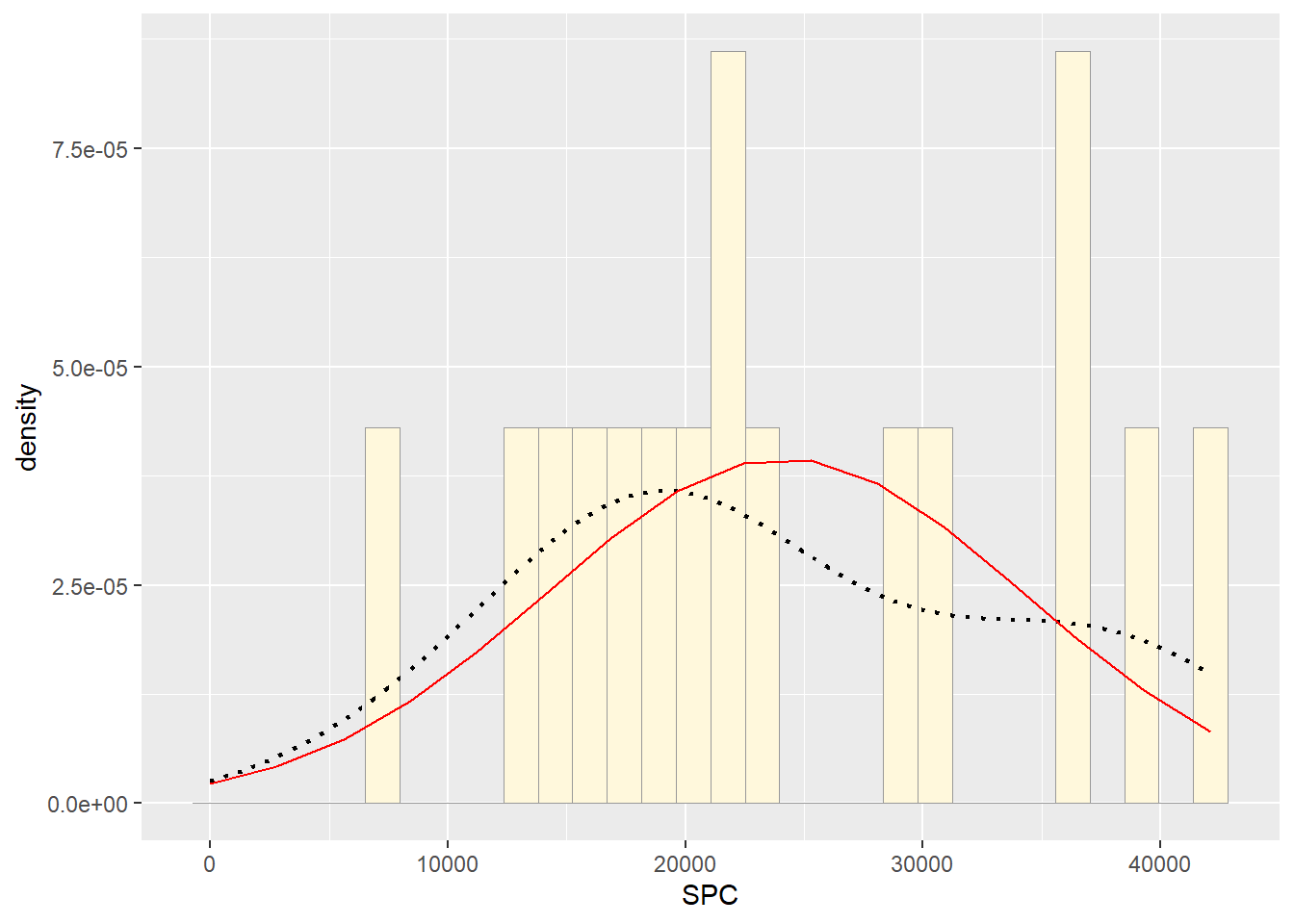
#Plot exponential probability density
expoPars <- fitdistr(Z$SPC,"exponential")
rateML <- expoPars$estimate["rate"]
stat2 <- stat_function(aes(x = xval, y = ..y..), fun = dexp, colour="blue", n = length(Z$SPC), args = list(rate=rateML))
p2 + stat + stat2## `stat_bin()` using `bins = 30`. Pick better value with `binwidth`.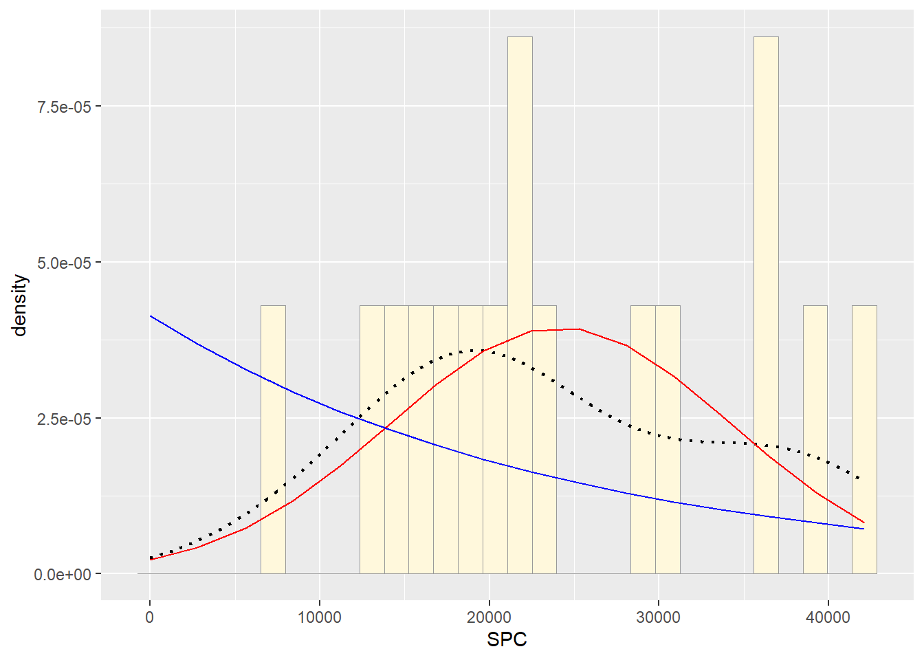 #Plot uniform probability density
stat3 <- stat_function(aes(x = xval, y = ..y..), fun = dunif, colour="darkgreen", n = length(Z$SPC), args = list(min=min(Z$SPC), max=max(Z$SPC)))
p2 + stat + stat2 + stat3## `stat_bin()` using `bins = 30`. Pick better value with `binwidth`.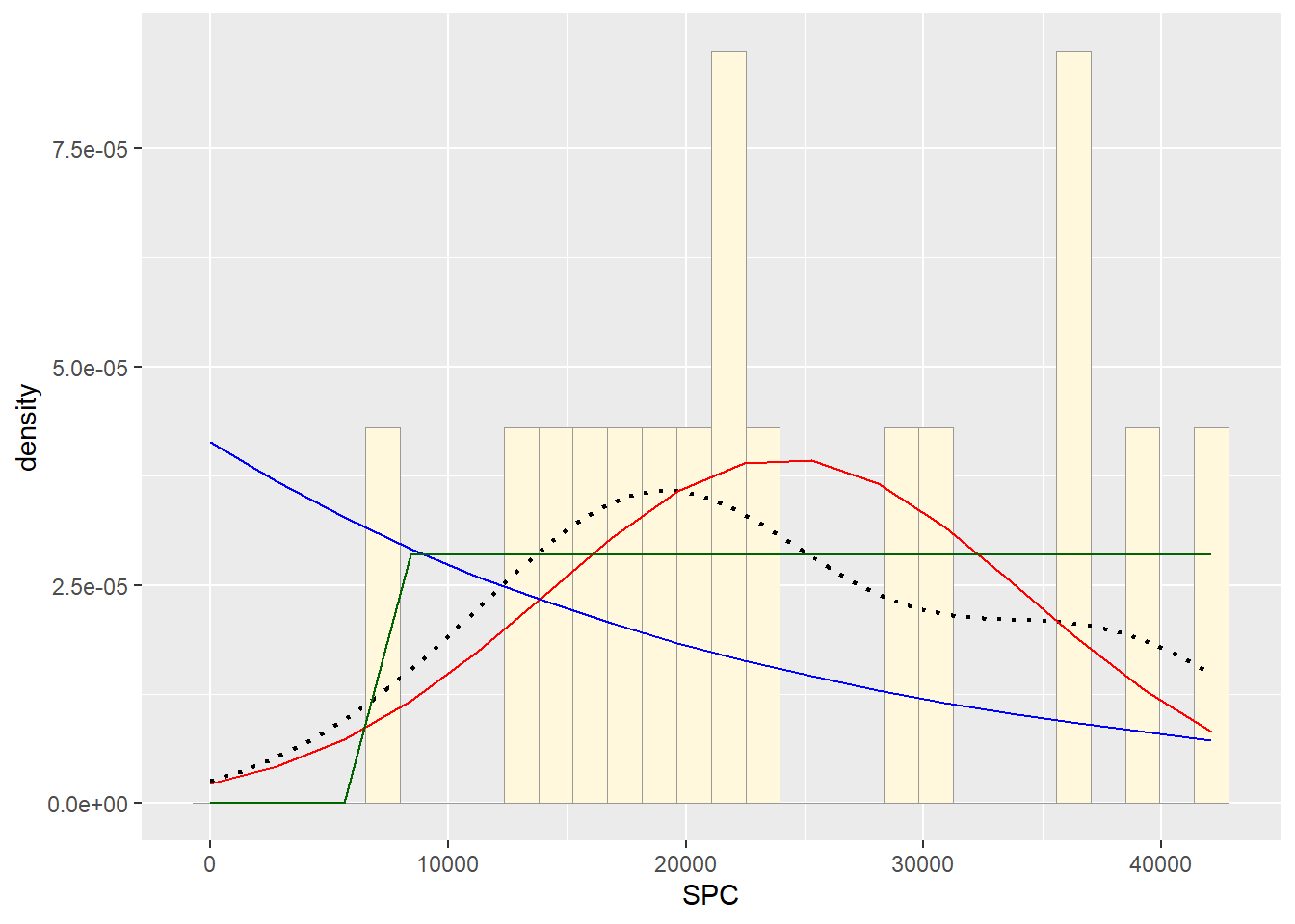 #Plot gamma probability density #observation:due to error from fitting,
defined the value of lower so it could run. For 0.001 was still giving
error.
#Plot gamma probability density #observation:due to error from fitting,
defined the value of lower so it could run. For 0.001 was still giving
error.
gammaPars <- fitdistr(Z$SPC,dgamma,list(shape=1,rate=0.1),lower=0.01)
shapeML <- gammaPars$estimate["shape"]
rateML <- gammaPars$estimate["rate"]
stat4 <- stat_function(aes(x = xval, y = ..y..), fun = dgamma, colour="brown", n = length(Z$SPC), args = list(shape=shapeML, rate=rateML))
p2 + stat + stat2 + stat3 + stat4## `stat_bin()` using `bins = 30`. Pick better value with `binwidth`.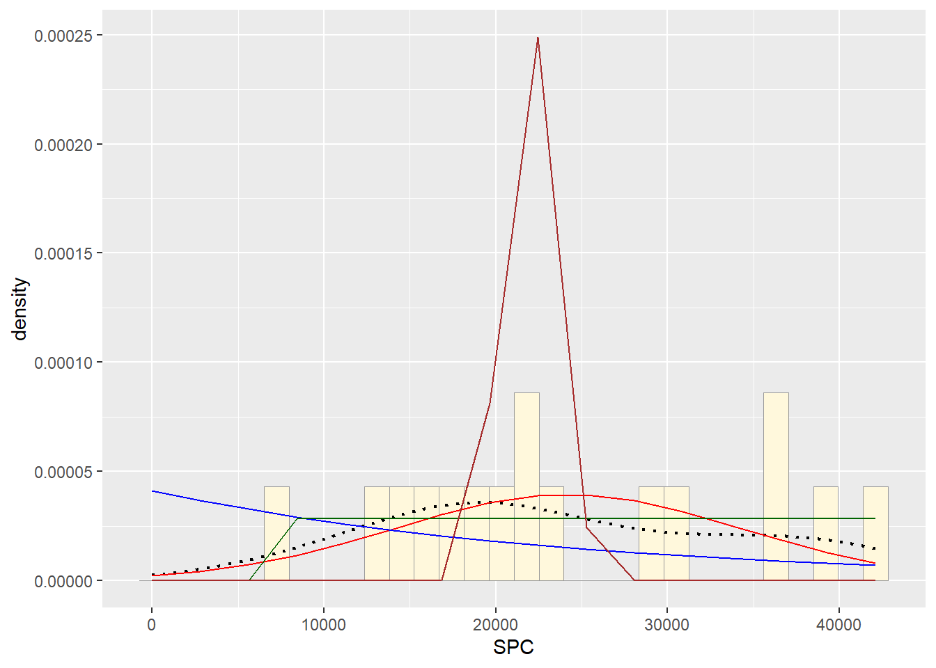 #Plot beta probability density
pSpecial <- ggplot(data=Z, aes(x=SPC/(max(SPC + 0.1)), y=..density..)) +
geom_histogram(color="grey60",fill="cornsilk",size=0.2) +
xlim(c(0,1)) +
geom_density(size=0.75,linetype="dotted")
betaPars <- fitdistr(x=Z$SPC/max(Z$SPC + 0.1),start=list(shape1=1,shape2=2),"beta")## Warning in densfun(x, parm[1], parm[2], ...): NaNs produzidos
## Warning in densfun(x, parm[1], parm[2], ...): NaNs produzidos
## Warning in densfun(x, parm[1], parm[2], ...): NaNs produzidos
## Warning in densfun(x, parm[1], parm[2], ...): NaNs produzidos
## Warning in densfun(x, parm[1], parm[2], ...): NaNs produzidosshape1ML <- betaPars$estimate["shape1"]
shape2ML <- betaPars$estimate["shape2"]
statSpecial <- stat_function(aes(x = xval, y = ..y..), fun = dbeta, colour="orchid", n = length(Z$SPC), args = list(shape1=shape1ML,shape2=shape2ML))
pSpecial + statSpecial## `stat_bin()` using `bins = 30`. Pick better value with `binwidth`.## Warning: Removed 2 rows containing missing values or values outside the scale range
## (`geom_bar()`).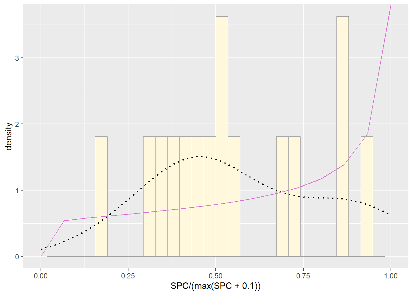
Although no fit was perfect, uniform distribution showed the best model for the data.